The durability of exposed geomembrane covers

The most frequently asked question by people in the geosynthetics world is how long is the anticipated lifetime of geosynthetics. So much so that of the more than 3,000 questions submitted to the GMA Techline since it began in 2004, 591 (19.7%) have been on lifetime, aka durability. Of these, 49% were on buried lifetime, and 30% were on exposed lifetime. This article addresses the exposed lifetime of five commercially available geomembranes. It is based on several high-temperature incubations of samples, which degrade over time and are quantified by evaluating loss of tensile strength and tensile elongation. When a 50% reduction is reached, the data is analyzed for half-life in a manner comparable to that used for all plastics (e.g., gas mains, cable shielding, plastic rope, etc.). This results in the predicted half-life under laboratory conditions. One additional step is taken, extending the laboratory data to a site-specific field site. For this article, Phoenix, Arizona, is arbitrarily selected. By using a ratio of radiation values in the laboratory compared to field radiation, such lifetimes are estimated.

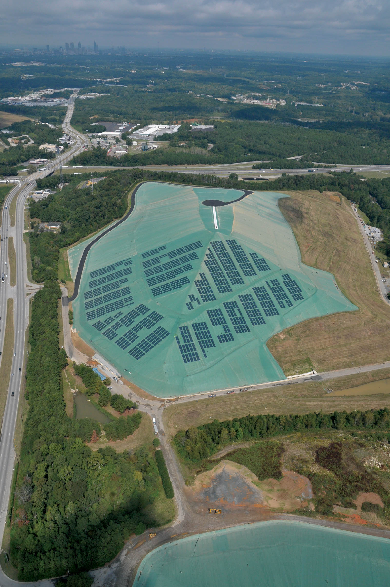
Figure 1 illustrates a case history of an exposed geomembrane cover on a landfill. There are many other cases as well (see Koerner 2011). Invariably, the anticipated service lifetime is asked by owners, regulators and designers, as well as by the suppliers, manufacturers and installers who are involved. Other than intentional or accidental damage, the possible degradation mechanisms are ultraviolet radiation, oxidation, hydrolysis, chemical, radioactive, biological, migration and temperature.

Each mechanism only has relevance depending on site-specific conditions as well as the specific type of geosynthetic resin and the formulation from which the geomembrane was made. If a specific mechanism is involved, testing organizations have appropriate standards for such laboratory evaluation. The results of such testing, however, are usually of a “go–no go” nature insofar as a final selection of material. They are not meant to be lifetime prediction methods.

To answer the lifetime question, the process is quite detailed and takes considerably longer. We use elevated temperature incubations followed by extrapolation to lower (presumably site-specific) temperatures for the prediction. It gives half-life times for the laboratory and field, both down to 680F (200C). Although Phoenix is used for the field conditions, the procedure is applicable wherever average ultraviolet radiation data is available.

Ultraviolet degradation and the method of incubation

Ultraviolet light (UV) is the major cause of degradation to all exposed organic materials. The UV region is subdivided into UV-A (400 to 315 nm), which causes some polymer damage; UV-B (315 to 280 nm), which causes severe polymer damage; and UV-C (280 to 100 nm), which is only found in outer space. Other factors in the degradation process of polymers are geographic location, temperature, cloud cover, wind, moisture, atmospheric pollution and product orientation. While difficult to assess, these should be considered for field lifetime prediction. Laboratory simulation is critical, however, for it provides the baseline degradation under completely controlled conditions of radiation, temperature, oxidation and moisture.

For laboratory simulation of sunlight, artificial light sources (lamps) are generally compared with worst-case conditions, or the solar maximum condition. The actual degradation is caused by photons of light breaking the polymer’s chemical bonds. For each type of bond, there is a threshold wavelength for bond scission, above which the bonds will not break and below it they will. Thus, the short wavelengths are critical. Van Zanten (1986) shows that polyethylene is most sensitive to UV degradation around 300 nm, polyvinyl chloride around 312 nm, polyester around 325 nm and polypropylene around 370 nm. That said, they are all within the UV-A or UV-B range of the wavelength spectrum.

Of the available laboratory weathering devices, the two most common are xenon arc (ASTM D4355) and ultraviolet fluorescent devices (ASTM D7238). Both devices incorporate UV radiation, oxidation, hydrolysis and high temperature. Everything else, particularly the original cost and maintenance costs, favors the UV-fluorescent device in the authors’ opinion. When considering that this study is a fourteen-year effort to date, the use of UV-fluorescent devices becomes an obvious choice at least in the context of this research project financed by the Geosynthetic Institute (GSI).

Whatever the incubation protocol, representative test samples are incubated and removed at periodic times, cut into tension test specimens, and evaluated for their retained strength and elongation. The results are then compared to the unexposed geomembrane for percent-retained values (see Koerner et al. 2017). When plotted and then extrapolated to lower temperatures, lifetime predictions in laboratory weathering devices can be obtained. Using this information, an extension to a specific field location can be generated, albeit with some quite serious assumptions. The specific procedure for the different geomembranes evaluated is as follows.

Methodology used and graphical example for half-life predictions

Used in this study are three separate devices set at 176°F (80°C), 158°F (70°C) and 140°F (60°C) constant temperatures. Each daily cycle is set for 20 hours lights on and four hours lights off, the latter being with water condensation. The lifetime prediction procedure that will be followed herein is accomplished in the three stages described below:

Step 1: Incubation Procedure

• Select a specific geomembrane material(s) to be investigated.
• Cut sample coupons for each incubation temperature to fit into the holders.
• Install these coupons in at least three different constant temperature incubation devices.
• Periodically remove coupons, die cut them into specimens, and test them for both tensile strength and elongation at break.
• Compare these gradually decreasing values to original values of nonincubated material for a percent strength and elongation retained, and plot the trends as incubation time versus percent retained.

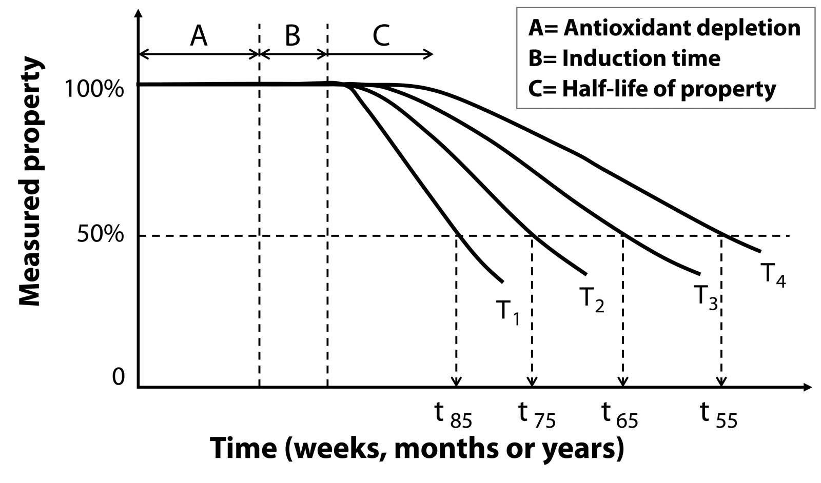
Step 2: Data Analysis to Reach Laboratory Lifetimes

• Select 50% retained values for both strength and elongation at each temperature; these are the so-called half-lives.
• Plot these three temperature data points
  on a semilogarithmic or arithmetic graph, and connect them using a least squares fitting method.
• Extrapolate the curves down to an arbitrarily selected temperature. A value of 68°F (20°C) will be used in all cases.
• This results in the half-life of strength and elongation under these specific laboratory incubation conditions.

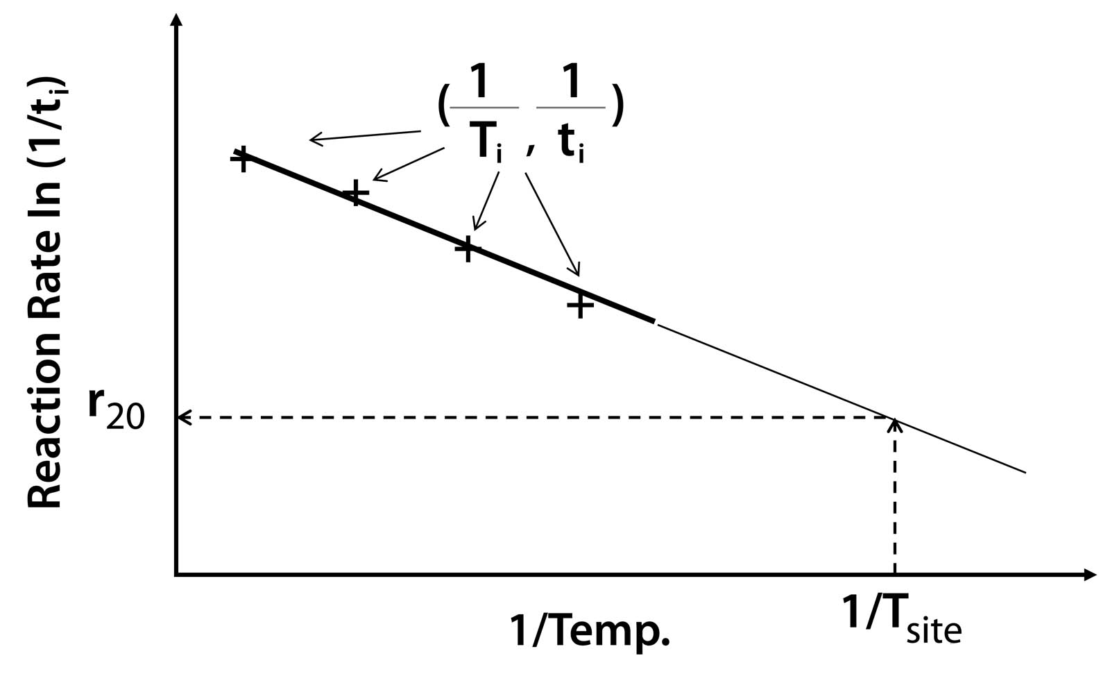
Step 3: Data Analysis to Reach Site-Specific Field Lifetimes

• Convert the measured half-life times in the laboratory at the three elevated temperatures to obtain total radiation energy values. This is a known value obtained from the weathering device manufacturer.
• Obtain the ultraviolet radiation at the field location of interest. This is also a known radiation value as obtained from national
  or world energy maps.
• Calculate the equivalent time to reach half-life at the field site using the appropriate field radiation.
• Plot these times using a least squares
  fitting method.
• Extrapolate down to 68°F (20°C) for half-life predictions based on these 50% loss-of-strength and elongation data points, and assess the results as well as make comparisons to the laboratory predicted values also at 68°F (20°C).

Half-life prediction values for five geomembranes

Accelerated aging was performed on five commercially available geomembranes (see Table 1). Their laboratory half-life calculations and the field half-life calculations were compared by generated plots as depicted in Figures 2 and 3.

Some commentary in regard to the selected geomembranes is appropriate. With the promulgation of the solid waste landfill regulations by the U.S. Environmental Protection Agency in 1982, geomembranes were required beneath and above the encapsulated solid waste mass. The regulations require the geomembrane thickness to be 0.75 mm, except for HDPE, which is required to be 1.50 mm thick.

The HDPE selected is black and conforms to the Geosynthetic Research Institute (GRI) GM13 generic specification. The standard oxidative induction time (OIT) value was 67.0 minutes (min), and its as-manufactured strength and elongation are given in Table 1 as with the other geomembranes.

Regarding the LLDPE selected, it was 1.0 mm thick. It is also black and conforms to the GRI GM17 generic specification. It has a standard OIT value of 21.1 min.

Regarding the fPP selected, it is a mixture, or blend, of polypropylene and a thermoset rubber and is best made in a reactor rather than blended in an extruder. This particular material is reactor grade. It is 1.0 mm, also black, has a standard OIT value of 7.2 min and conforms to the GRI GM18 generic specification.

Regarding the EPDM selected, it is a thermoset polymer, also 1.0 mm thick, black and conforms to the GRI GM21 generic specification. It has no antioxidants in the formulation.

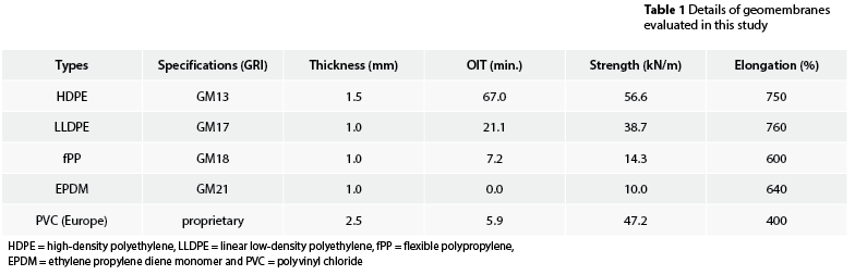
Lastly, the PVC that is customarily used in North America follows ASTM D7176, but this standard specification states that it is to be “used in buried applications.” As a result, we selected a European PVC formulation that has been successfully used for more than 40 years when exposed in waterproofing dams; see Scuero and Vaschetti (1996) and Cazzuffi (2014). It is 2.5 mm thick, gray and is only available via the manufacturer’s proprietary specification. It has antioxidants with OIT of 5.9 min and several high molecular weight plasticizers that are proprietary.

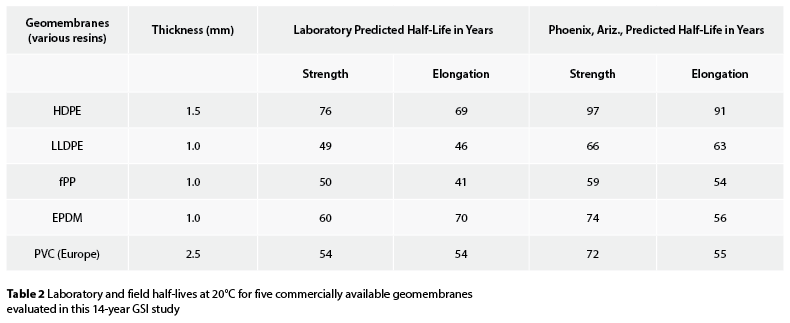
The resulting half-life prediction values obtained for the five geomembranes evaluated in this study are presented in Table 2. In each case, strength and elongation half-lives are given for both laboratory and field results.

In viewing the response curves after incubation and the calculated half-lives of laboratory and field projections as shown in Table 2, the following is observed regarding the results of the five geomembranes that were evaluated. See Koerner et al. (2017) for greater detail.

The strength and elongation retained curves versus incubation times are reasonably well behaved considering that each data point is at a specific incubation time.

The HDPE results in the longest half-life values in both the laboratory and field situations. That said, its thickness is slightly greater than the others, except for the PVC (Europe). In addition, the other four geomembranes have somewhat similar half-life values. Note that there are reverses of strength half-lives and elongation half-lives within the various geomembranes. As an overall comment, the field half-lives are greater than laboratory half-lives.

Conclusions

Geomembranes have shown themselves to be long-lasting exposed landfill covers. This application of exposed geomembrane covers in landfill designs has resulted in significant savings in construction costs and capacity. Operating with an exposed geomembrane cover, landfill gas recovery and solar-generated electricity are readily accommodated. Of particular note is that all field-predicted values in Table 2 exceed the U.S. EPA regulations mentioned earlier of requiring a 30-year final cover-care period.

It needs to be made clear that the type of geomembrane and its specific formulation is of considerable importance to its longevity as an exposed geomembrane cover. The difference between the very long lifetimes when covered (see Koerner 2012) versus the much shorter times when exposed are due to three main degradation mechanisms: ultraviolet radiation, high temperatures and full atmospheric oxidation.

In conclusion, it is felt that this type of lifetime prediction for exposed geomembranes is reasonably simulated in laboratory weathering devices. While such laboratory lifetimes are of value in comparing different products or different formulations of the same product, the process can also be used to compare to a given specification. That said, the extension of laboratory to field lifetime prediction is much more subjective.

Acknowledgments

This research project was sponsored by the members of the Geosynthetic Institute. As such, the authors sincerely appreciate the current and past members, affiliated members and associate members. The current member list is available on the GSI website (http://www.geosynthetic-institute.org).

George R. Koerner, Ph.D., P.E., C.Q.A., is the director of the Geosynthetic Institute in Folsom, Pa.

Robert M. Koerner, Ph.D., is a professor emeritus of civil engineering at Drexel University in Philadelphia, Pa., the author of Designing with Geosynthetics in multiple editions and a pioneer in the development of geosynthetics as a construction material.

Y. Grace Hsuan, Ph.D., is a professor of civil, environmental and architectural engineering at Drexel University in Philadelphia, Pa. She is also the associate director of the Geosynthetic Research Institute in Folsom, Pa.